This Quantum world/Print version

[[Category:Books with print version|Template:BOOKNAME]]

What does an atom look like?

Like this?

• File:Barium (Elektronenbestzung).png
• 
• 

Image on left is public domain. Second from left is GFDL by Wikimedia Commons users Jeanot and Svdmolen. Image on right by Wikimedia Commons user Halfdan (also GFDL).

Or like this?

• 
  ${\rho }_{2p0}$
• 
  ${\rho }_{3p0}$
• 
  ${\rho }_{3d0}$
• 
  ${\rho }_{4p0}$
• 
  ${\rho }_{4d0}$
• 
  ${\rho }_{4f0}$
• 
  ${\rho }_{5d0}$
• 
  ${\rho }_{5f0}$

All of the above gallery of images by Ulrich Mohrhoff and created with David Manthey's free Orbital Viewer

None of these images depicts an atom as it is. This is because it is impossible to even visualize an atom as it is. Whereas the best you can do with the images in the first row is to erase them from your memory, the eight fuzzy images in the next two rows deserve scrutiny. Each represents an aspect of a stationary state of atomic hydrogen. You see neither the nucleus (a proton) nor the electron. What you see is a fuzzy position. To be precise, what you see is a cloudlike blur, which is symmetrical about the vertical axis, and which represents the atom's internal relative position — the position of the electron relative to the proton or the position of the proton relative to the electron.

• What is the state of an atom?
• What is a stationary state?
• What exactly is a fuzzy position?
• How does such a blur represent the atom's internal relative position?
• Why can we not describe the atom's internal relative position as it is?

Quantum states

In quantum mechanics, states are probability algorithms. We use them to calculate the probabilities of the possible outcomes of measurements on the basis of actual measurement outcomes. A quantum state takes as its input

• one or several measurement outcomes,
• a measurement M,
• the time of M,

and it yields as its output the probabilities of the possible outcomes of M.

A quantum state is called stationary if the probabilities it assigns are independent of the time of the measurement to the possible outcomes of which they are assigned.

From the mathematical point of view, each blur represents a density function $\rho (𝒓)$. Imagine a small region $R$ like the little box inside the first blur. And suppose that this is a region of the (mathematical) space of positions relative to the proton. If you integrate $\rho (𝒓)$ over $R,$ you obtain the probability $p(R)$ of finding the electron in $R,$ provided that the appropriate measurement is made:

$p(R)=\underset{R}{\int }\rho (𝒓)d^3𝒓.$

"Appropriate" here means capable of ascertaining the truth value of the proposition "the electron is in $R$", the possible truth values being "true" or "false". What we see in each of the following images is a surface of constant probability density.

• 
  ${\rho }_{2p0}$
• 
  ${\rho }_{3p0}$
• 
  ${\rho }_{3d0}$
• 
  ${\rho }_{4p0}$
• 
  ${\rho }_{4d0}$
• 
  ${\rho }_{4f0}$
• 
  ${\rho }_{5d0}$
• 
  ${\rho }_{5f0}$

All of the above gallery of images by Ulrich Mohrhoff and created with David Manthey's free Orbital Viewer

Now imagine that the appropriate measurement is made. Before the measurement, the electron is neither inside $R$ nor outside $R,$ for if it were inside, the probability of finding it outside would be zero, and if it were outside, the probability of finding it inside would be zero. After the measurement, on the other hand, the electron is either inside or outside $R.$

Conclusions:

• Before the measurement, the proposition "the electron is in $R$" is neither true nor false; it lacks a (definite) truth value.
• A measurement generally changes the state of the system on which it is performed.

As mentioned before, probabilities are assigned not only to measurement outcomes but also on the basis of measurement outcomes. Each density function ${\rho }_{nlm}$ serves to assign probabilities to the possible outcomes of a measurement of the position of the electron relative to the proton. And in each case the assignment is based on the outcomes of a simultaneous measurement of three observables: the atom's energy (specified by the value of the principal quantum number $n$), its total angular momentum $l$ (specified by a letter, here p, d, or f), and the vertical component of its angular momentum $m$.

Fuzzy observables

We say that an observable $Q$ with a finite or countable number of possible values $q_k$ is fuzzy (or that it has a fuzzy value) if and only if at least one of the propositions "The value of $Q$ is $q_k$" lacks a truth value. This is equivalent to the following necessary and sufficient condition: the probability assigned to at least one of the values $q_k$ is neither 0 nor 1.

What about observables that are generally described as continuous, like a position?

The description of an observable as "continuous" is potentially misleading. For one thing, we cannot separate an observable and its possible values from a measurement and its possible outcomes, and a measurement with an uncountable set of possible outcomes is not even in principle possible. For another, there is not a single observable called "position". Different partitions of space define different position measurements with different sets of possible outcomes.

• Corollary: The possible outcomes of a position measurement (or the possible values of a position observable) are defined by a partition of space. They make up a finite or countable set of regions of space. An exact position is therefore neither a possible measurement outcome nor a possible value of a position observable.

So how do those cloudlike blurs represent the electron's fuzzy position relative to the proton? Strictly speaking, they graphically represent probability densities in the mathematical space of exact relative positions, rather than fuzzy positions. It is these probability densities that represent fuzzy positions by allowing us to calculate the probability of every possible value of every position observable.

It should now be clear why we cannot describe the atom's internal relative position as it is. To describe a fuzzy observable is to assign probabilities to the possible outcomes of a measurement. But a description that rests on the assumption that a measurement is made, does not describe an observable as it is (by itself, regardless of measurements).

Serious illnesses require drastic remedies

Planck

Quantum mechanics began as a desperate measure to get around some spectacular failures of what subsequently came to be known as classical physics.

In 1900 Max Planck discovered a law that perfectly describes the spectrum of a glowing hot object. Planck's radiation formula turned out to be irreconcilable with the physics of his time. (If classical physics were right, you would be blinded by ultraviolet light if you looked at the burner of a stove.) At first, it was just a fit to the data, "a fortuitous guess at an interpolation formula" as Planck himself called it. Only weeks later did it turn out to imply the quantization of energy for the emission of electromagnetic radiation: the energy $E$ of a quantum of radiation is proportional to the frequency $\nu$ of the radiation, the constant of proportionality being Planck's constant $h$:

$E=h\nu$.

We can of course use the angular frequency $\omega =2\pi \nu$ instead of $\nu$. Introducing the reduced Planck constant $\hslash =h/2\pi$, we then have

$E=\hslash \omega$.

Rutherford

In 1911 Ernest Rutherford proposed a model of the atom based on experiments by Geiger and Marsden. Geiger and Marsden had directed a beam of alpha particles at a thin gold foil. Most of the particles passed the foil more or less as expected, but about one in 8000 bounced back as if it had encountered a much heavier object. In Rutherford's own words this was as incredible as if you fired a 15 inch cannon ball at a piece of tissue paper and it came back and hit you. After analysing the data collected by Geiger and Marsden, Rutherford concluded that the diameter of the atomic nucleus (which contains over 99.9% of the atom's mass) was less that 0.01% of the diameter of the entire atom, and he suggested that atomic electrons orbit the nucleus much like planets orbit a star.

Classical electromagnetic theory, however, predicts that an orbiting electron will radiate away its energy and spiral into the nucleus in about 0.0000000005 of a second. This was the worst quantitative failure in the history of physics, under-predicting the lifetime of hydrogen by at least forty orders of magnitude! (This figure is based on the experimentally established lower bound on the proton's lifetime.)

Bohr

In 1913 Niels Bohr postulated that the angular momentum $L$ of an orbiting atomic electron was quantized: its "allowed" values are integral multiples of $\hslash$:

$L=n\hslash$ where $n=1,2,3,\dots$

Why quantize angular momentum, rather than any other quantity?

• Radiation energy of a given frequency is quantized in multiples of Planck's constant.
• Planck's constant is measured in the same units as angular momentum.

Bohr's postulate explained not only the stability of atoms but also why the emission and absorption of electromagnetic radiation by atoms is discrete. In addition it enabled him to calculate with remarkable accuracy the spectrum of atomic hydrogen — the frequencies at which it is able to emit and absorb light (visible as well as infrared and ultraviolet). The following image shows the visible emission spectrum of atomic hydrogen, which contains four lines of the Balmer series.

Visible emission spectrum of atomic hydrogen, containing four lines of the Balmer series. . This image is in the Public Domain

GFDL Licensed Image by Ulrich Mohrhoff

Apart from his quantization postulate, Bohr's reasoning at this point remained completely classical. Let's assume with Bohr that the electron's orbit is a circle of radius $r.$ The speed of the electron is then given by $v=rd\beta /dt,$ and the magnitude of its acceleration by $a=dv/dt=vd\beta /dt.$ Eliminating $d\beta /dt$ yields $a=v^2/r.$ In the cgs system of units, the magnitude of the Coulomb force is simply $F=e^2/r^2,$ where $e$ is the magnitude of the charge of both the electron and the proton. Via Newton's $F=ma$ the last two equations yield $m_e{v}^2=e^2/r,$ where $m_e$ is the electron's mass. If we take the proton to be at rest, we obtain $T=m_e{v}^2/2=e^2/2r$ for the electron's kinetic energy.

If the electron's potential energy at infinity is set to 0, then its potential energy $V$ at a distance $r$ from the proton is minus the work required to move it from $r$ to infinity,

$V=-\underset{r}{\overset{\mathrm{\infty }}{\int }}Fdr=-\underset{r}{\overset{\mathrm{\infty }}{\int }}\frac{e^2}{(r^{\prime }{)}^2}d{r}^{\prime }=+{\left[\frac{e^2}{r^{\prime }}\right]}_r^{\mathrm{\infty }}=0-\frac{e^2}{r}.$

The total energy of the electron thus is

$E=T+V=e^2/2r-e^2/r=-e^2/2r.$

We want to express this in terms of the electron's angular momentum $L=m_{e}vr.$ Remembering that $m_e{v}^2=e^2/r,$ and hence $r{m}_e^2{v}^2=m_e{e}^2,$ and multiplying the numerator $e^2$ by $m_e{e}^2$ and the denominator $2r$ by $r{m}_e^2{v}^2,$ we obtain

$E=-\frac{e^2}{2r}=-\frac{m_e{e}^4}{2m_e^2{v}^2{r}^2}=-\frac{m_e{e}^4}{2L^2}.$

Now comes Bohr's break with classical physics: he simply replaced $L$ by $n\hslash$. The "allowed" values for the angular momentum define a series of allowed values for the atom's energy:

$E_n=-\frac{1}{n^2}\left(\frac{m_e{e}^4}{2{\hslash }^2}\right),n=1,2,3,\dots$

As a result, the atom can emit or absorb energy only by amounts equal to the absolute values of the differences

$\mathrm{\Delta }{E}_{nm}=E_n-E_m=(\frac{1}{n^2}-\frac{1}{m^2})\text{Ry},$

one Rydberg (Ry) being equal to $m_e{e}^4/2{\hslash }^2=13.6056923(12)\text{eV.}$ This is also the ionization energy $\mathrm{\Delta }{E}_{1\mathrm{\infty }}$ of atomic hydrogen — the energy needed to completely remove the electron from the proton. Bohr's predicted value was found to be in excellent agreement with the measured value.

Using two of the above expressions for the atom's energy and solving for $r,$ we obtain $r=n^2{\hslash }^2/m_e{e}^2.$ For the ground state $(n=1)$ this is the Bohr radius of the hydrogen atom, which equals ${\hslash }^2/m_e{e}^2=5.291772108(18)\times 10^{-11}m.$ The mature theory yields the same figure but interprets it as the most likely distance from the proton at which the electron would be found if its distance from the proton were measured.

de Broglie

In 1923, ten years after Bohr had derived the spectrum of atomic hydrogen by postulating the quantization of angular momentum, Louis de Broglie hit on an explanation of why the atom's angular momentum comes in multiples of $\hslash .$ Since 1905, Einstein had argued that electromagnetic radiation itself was quantized (and not merely its emission and absorption, as Planck held). If electromagnetic waves can behave like particles (now known as photons), de Broglie reasoned, why cannot electrons behave like waves?

Suppose that the electron in a hydrogen atom is a standing wave on what has so far been thought of as the electron's circular orbit. (The crests, troughs, and nodes of a standing wave are stationary.) For such a wave to exist on a circle, the circumference of the latter must be an integral multiple of the wavelength $\lambda$ of the former: $2\pi r=n\lambda .$

• 
• 
• 
• 

The above images are GFDL Licensed Images by Ulrich Mohrhoff
Einstein had established not only that electromagnetic radiation of frequency $\nu$ comes in quanta of energy $E=h\nu$ but also that these quanta carry a momentum $p=h/\lambda .$ Using this formula to eliminate $\lambda$ from the condition $2\pi r=n\lambda ,$ one obtains $pr=n\hslash .$ But $pr=mvr$ is just the angular momentum $L$ of a classical electron with an orbit of radius $r.$ In this way de Broglie derived the condition $L=n\hslash$ that Bohr had simply postulated.

Schrödinger

If the electron is a standing wave, why should it be confined to a circle? After de Broglie's crucial insight that particles are waves of some sort, it took less than three years for the mature quantum theory to be found, not once but twice, by Werner Heisenberg in 1925 and by Erwin Schrödinger in 1926. If we let the electron to be a standing wave in three dimensions, we have all it takes to arrive at the Schrödinger equation, which is at the heart of the mature theory.

Let's keep to one spatial dimension. The simplest mathematical description of a wave of angular wavenumber $k=2\pi /\lambda$ and angular frequency $\omega =2\pi /T=2\pi \nu$ (at any rate, if you are familiar with complex numbers) is the function

$\psi (x,t)=e^{i(kx-\omega t)}.$

Let's express the phase $\varphi (x,t)=kx-\omega t$ in terms of the electron's energy $E=h\nu =\hslash \omega$ and momentum $p=h/\lambda =\hslash k:$

$\psi (x,t)=e^{i(px-Et)/\hslash }.$

The partial derivatives with respect to $x$ and $t$ are

$\frac{\partial \psi }{\partial x}=\frac{i}{\hslash }p\psi \text{and}\frac{\partial \psi }{\partial t}=-\frac{i}{\hslash }E\psi .$

We also need the second partial derivative of $\psi$ with respect to $x$:

$\frac{{\partial }^2\psi }{\partial x^2}={\left(\frac{ip}{\hslash }\right)}^2\psi .$

We thus have

$E\psi =i\hslash \frac{\partial \psi }{\partial t},p\psi =-i\hslash \frac{\partial \psi }{\partial x},\text{and}{p}^2\psi =-{\hslash }^2\frac{{\partial }^2\psi }{\partial x^2}.$

In non-relativistic classical physics the kinetic energy and the kinetic momentum $p$ of a free particle are related via the dispersion relation

$E=p^2/2m.$

This relation also holds in non-relativistic quantum physics. Later you will learn why.

In three spatial dimensions, $p$ is the magnitude of a vector $\mathbf{\text{p}}.$ If the particle also has a potential energy $V(\mathbf{\text{r}},t)$ and a potential momentum $\mathbf{\text{A}}(\mathbf{\text{r}},t)$ (in which case it is not free), and if $E$ and $\mathbf{\text{p}}$ stand for the particle's total energy and total momentum, respectively, then the dispersion relation is

$E-V=(\mathbf{\text{p}}-\mathbf{\text{A}}{)}^2/2m.$

By the square of a vector $\mathbf{\text{v}}$ we mean the dot (or scalar) product $\mathbf{\text{v}}\cdot \mathbf{\text{v}}$. Later you will learn why we represent possible influences on the motion of a particle by such fields as $V(\mathbf{\text{r}},t)$ and $\mathbf{\text{A}}(\mathbf{\text{r}},t).$

Returning to our fictitious world with only one spatial dimension, allowing for a potential energy $V(x,t)$, substituting the differential operators $i\hslash \frac{\partial }{\partial t}$ and $-{\hslash }^2\frac{{\partial }^2}{\partial x^2}$ for $E$ and $p^2$ in the resulting dispersion relation, and applying both sides of the resulting operator equation to $\psi ,$ we arrive at the one-dimensional (time-dependent) Schrödinger equation:

$i\hslash \frac{\partial \psi }{\partial t}=-\frac{{\hslash }^2}{2m}\frac{{\partial }^2\psi }{\partial x^2}+V\psi$

In three spatial dimensions and with both potential energy $V(\mathbf{\text{r}},t)$ and potential momentum $\mathbf{\text{A}}(\mathbf{\text{r}},t)$ present, we proceed from the relation $E-V=(\mathbf{\text{p}}-\mathbf{\text{A}}{)}^2/2m,$ substituting $i\hslash \frac{\partial }{\partial t}$ for $E$ and $-i\hslash \frac{\partial }{\partial \mathbf{\text{r}}}$ for $\mathbf{\text{p}}.$ The differential operator $\frac{\partial }{\partial \mathbf{\text{r}}}$ is a vector whose components are the differential operators $(\frac{\partial \psi }{\partial x},\frac{\partial \psi }{\partial y},\frac{\partial \psi }{\partial z}).$ The result:

$i\hslash \frac{\partial \psi }{\partial t}=\frac{1}{2m}{(-i\hslash \frac{\partial }{\partial \mathbf{\text{r}}}-\mathbf{\text{A}})}^2\psi +V\psi ,$

where $\psi$ is now a function of $\mathbf{\text{r}}=(x,y,z)$ and $t.$ This is the three-dimensional Schrödinger equation. In non-relativistic investigations (to which the Schrödinger equation is confined) the potential momentum can generally be ignored, which is why the Schrödinger equation is often given this form:

$i\hslash \frac{\partial \psi }{\partial t}=-\frac{{\hslash }^2}{2m}(\frac{{\partial }^2\psi }{\partial x^2}+\frac{{\partial }^2\psi }{\partial y^2}+\frac{{\partial }^2\psi }{\partial z^2})+V\psi$

The free Schrödinger equation (without even the potential energy term) is satisfied by $\psi (x,t)=e^{i(kx-\omega t)}$ (in one dimension) or $\psi (\mathbf{\text{r}},t)=e^{i(𝐤\cdot 𝐫-\omega t)}$ (in three dimensions) provided that $E=\hslash \omega$ equals $p^2/2m=(\hslash k{)}^2/2m,$ which is to say: $\omega (k)=\hslash k^2/2m.$ However, since we are dealing with a homogeneous linear differential equation — which tells us that solutions may be added and/or multiplied by an arbitrary constant to yield additional solutions — any function of the form

$\psi (x,t)=\frac{1}{\sqrt{2\pi }}\int \bar{\psi }(k)e^{i[kx-\omega (k)t]}dk=\frac{1}{\sqrt{2\pi }}\int \bar{\psi }(k,t)e^{ikx}dk$

with $\bar{\psi }(k,t)=\bar{\psi }(k)e^{-i\omega (k)t}$ solves the (one-dimensional) Schrödinger equation. If no integration boundaries are specified, then we integrate over the real line, i.e., the integral is defined as the limit $\underset{L\to \mathrm{\infty }}{\lim }\underset{-L}{\overset{+L}{\int }}.$ The converse also holds: every solution is of this form. The factor in front of the integral is present for purely cosmetic reasons, as you will realize presently. $\bar{\psi }(k,t)$ is the Fourier transform of $\psi (x,t),$ which means that

$\bar{\psi }(k,t)=\frac{1}{\sqrt{2\pi }}\int \psi (x,t)e^{-ikx}dx.$

The Fourier transform of $\psi (x,t)$ exists because the integral $\int |\psi (x,t)|dx$ is finite. In the next section we will come to know the physical reason why this integral is finite.

So now we have a condition that every electron "wave function" must satisfy in order to satisfy the appropriate dispersion relation. If this (and hence the Schrödinger equation) contains either or both of the potentials $V$ and $\mathbf{\text{A}}$, then finding solutions can be tough. As a budding quantum mechanician, you will spend a considerable amount of time learning to solve the Schrödinger equation with various potentials.

Born

In the same year that Erwin Schrödinger published the equation that now bears his name, the nonrelativistic theory was completed by Max Born's insight that the Schrödinger wave function $\psi (𝐫,t)$ is actually nothing but a tool for calculating probabilities, and that the probability of detecting a particle "described by" $\psi (𝐫,t)$ in a region of space $R$ is given by the volume integral

$\underset{R}{\int }|\psi (t,𝐫){|}^2{d}^{3}r=\underset{R}{\int }{\psi }^{*}\psi d^{3}r$

— provided that the appropriate measurement is made, in this case a test for the particle's presence in $R$. Since the probability of finding the particle somewhere (no matter where) has to be 1, only a square integrable function can "describe" a particle. This rules out $\psi (𝐫)=e^{i𝐤\cdot 𝐫},$ which is not square integrable. In other words, no particle can have a momentum so sharp as to be given by $\hslash$ times a wave vector $𝐤$, rather than by a genuine probability distribution over different momenta.

Given a probability density function $|\psi (x){|}^2$, we can define the expected value

$⟨x⟩=\int |\psi (x){|}^{2}xdx=\int {\psi }^{*}x\psi dx$

and the standard deviation  $\mathrm{\Delta }x=\sqrt{\int |\psi {|}^2(x-⟨x⟩{)}^2}$

as well as higher moments of $|\psi (x){|}^2$. By the same token,

$⟨k⟩=\int \bar{\psi }{}^{*}k\bar{\psi }dk$  and  $\mathrm{\Delta }k=\sqrt{\int |\bar{\psi }{|}^2(k-⟨k⟩{)}^2}.$

Here is another expression for $⟨k⟩:$

$⟨k⟩=\int {\psi }^{*}(x)(-i\frac{d}{dx})\psi (x)dx.$

To check that the two expressions are in fact equal, we plug  $\psi (x)=(2\pi {)}^{-1/2}\int \bar{\psi }(k)e^{ikx}dk$  into the latter expression:

$⟨k⟩=\frac{1}{\sqrt{2\pi }}\int {\psi }^{*}(x)(-i\frac{d}{dx})\int \bar{\psi }(k)e^{ikx}dkdx=\frac{1}{\sqrt{2\pi }}\int {\psi }^{*}(x)\int \bar{\psi }(k)k{e}^{ikx}dkdx.$

Next we replace ${\psi }^{*}(x)$ by $(2\pi {)}^{-1/2}\int \bar{\psi }{}^{*}(k^{\prime })e^{-i{k}^{\prime }x}d{k}^{\prime }$  and shuffle the integrals with the mathematical nonchalance that is common in physics:

$⟨k⟩=\int \int \bar{\psi }{}^{*}(k^{\prime })k\bar{\psi }(k)[\frac{1}{2\pi }\int e^{i(k-k^{\prime })x}dx]dkd{k}^{\prime }.$

The expression in square brackets is a representation of Dirac's delta distribution $\delta (k-k^{\prime }),$ the defining characteristic of which is  $\underset{-\mathrm{\infty }}{\overset{+\mathrm{\infty }}{\int }}f(x)\delta (x)dx=f(0)$  for any continuous function $f(x).$ (In case you didn't notice, this proves what was to be proved.)

Heisenberg

In the same annus mirabilis of quantum mechanics, 1926, Werner Heisenberg proved the so-called "uncertainty" relation

$\mathrm{\Delta }x\mathrm{\Delta }p\ge \hslash /2.$

Heisenberg spoke of Unschärfe, the literal translation of which is "fuzziness" rather than "uncertainty". Since the relation $\mathrm{\Delta }x\mathrm{\Delta }k\ge 1/2$ is a consequence of the fact that $\psi (x)$ and $\bar{\psi }(k)$ are related to each other via a Fourier transformation, we leave the proof to the mathematicians. The fuzziness relation for position and momentum follows via $p=\hslash k$. It says that the fuzziness of a position (as measured by $\mathrm{\Delta }x$ ) and the fuzziness of the corresponding momentum (as measured by $\mathrm{\Delta }p=\hslash \mathrm{\Delta }k$ ) must be such that their product equals at least $\hslash /2.$

The Feynman route to Schrödinger

The probabilities of the possible outcomes of measurements performed at a time $t_2$ are determined by the Schrödinger wave function $\psi (𝐫,t_2)$. The wave function $\psi (𝐫,t_2)$ is determined via the Schrödinger equation by $\psi (𝐫,t_1).$ What determines $\psi (𝐫,t_1)$ ? Why, the outcome of a measurement performed at $t_1$ — what else? Actual measurement outcomes determine the probabilities of possible measurement outcomes.

Two rules

In this chapter we develop the quantum-mechanical probability algorithm from two fundamental rules. To begin with, two definitions:

• Alternatives are possible sequences of measurement outcomes.
• With each alternative is associated a complex number called amplitude.

Suppose that you want to calculate the probability of a possible outcome of a measurement given the actual outcome of an earlier measurement. Here is what you have to do:

• Choose any sequence of measurements that may be made in the meantime.
• Assign an amplitude to each alternative.
• Apply either of the following rules:

Rule A: If the intermediate measurements are made (or if it is possible to infer from other measurements what their outcomes would have been if they had been made), first square the absolute values of the amplitudes of the alternatives and then add the results.

Rule B: If the intermediate measurements are not made (and if it is not possible to infer from other measurements what their outcomes would have been), first add the amplitudes of the alternatives and then square the absolute value of the result.

In subsequent sections we will explore the consequences of these rules for a variety of setups, and we will think about their origin — their raison d'être. Here we shall use Rule B to determine the interpretation of $\bar{\psi }(k)$ given Born's probabilistic interpretation of $\psi (x)$.

In the so-called "continuum normalization", the unphysical limit of a particle with a sharp momentum $\hslash k^{\prime }$ is associated with the wave function

${\psi }_{k^{\prime }}(x,t)=\frac{1}{\sqrt{2\pi }}\int \delta (k-k^{\prime })e^{i[kx-\omega (k)t]}dk=\frac{1}{\sqrt{2\pi }}{e}^{i[k^{\prime }x-\omega (k^{\prime })t]}.$

Hence we may write $\psi (x,t)=\int \bar{\psi }(k){\psi }_k(x,t)dk.$

$\bar{\psi }(k)$ is the amplitude for the outcome $\hslash k$ of an infinitely precise momentum measurement. ${\psi }_k(x,t)$ is the amplitude for the outcome $x$ of an infinitely precise position measurement performed (at time t) subsequent to an infinitely precise momentum measurement with outcome $\hslash k.$ And $\psi (x,t)$ is the amplitude for obtaining $x$ by an infinitely precise position measurement performed at time $t.$

The preceding equation therefore tells us that the amplitude for finding $x$ at $t$ is the product of

1. the amplitude for the outcome $\hslash k$ and
2. the amplitude for the outcome $x$ (at time $t$) subsequent to a momentum measurement with outcome $\hslash k,$

summed over all values of $k.$

Under the conditions stipulated by Rule A, we would have instead that the probability for finding $x$ at $t$ is the product of

1. the probability for the outcome $\hslash k$ and
2. the probability for the outcome $x$ (at time $t$) subsequent to a momentum measurement with outcome $\hslash k,$

summed over all values of $k.$

The latter is what we expect on the basis of standard probability theory. But if this holds under the conditions stipulated by Rule A, then the same holds with "amplitude" substituted from "probability" under the conditions stipulated by Rule B. Hence, given that ${\psi }_k(x,t)$ and $\psi (x,t)$ are amplitudes for obtaining the outcome $x$ in an infinitely precise position measurement, $\bar{\psi }(k)$ is the amplitude for obtaining the outcome $\hslash k$ in an infinitely precise momentum measurement.

Notes:

1. Since Rule B stipulates that the momentum measurement is not actually made, we need not worry about the impossibility of making an infinitely precise momentum measurement.
2. If we refer to $|\psi (x){|}^2$ as "the probability of obtaining the outcome $x,$" what we mean is that $|\psi (x){|}^2$ integrated over any interval or subset of the real line is the probability of finding our particle in this interval or subset.

An experiment with two slits

The setup

In this experiment, the final measurement (to the possible outcomes of which probabilities are assigned) is the detection of an electron at the backdrop, by a detector situated at D (D being a particular value of x). The initial measurement outcome, on the basis of which probabilities are assigned, is the launch of an electron by an electron gun G. (Since we assume that G is the only source of free electrons, the detection of an electron behind the slit plate also indicates the launch of an electron in front of the slit plate.) The alternatives or possible intermediate outcomes are

• the electron went through the left slit (L),
• the electron went through the right slit (R).

The corresponding amplitudes are $A_L$ and $A_R.$

Here is what we need to know in order to calculate them:

• $A_L$ is the product of two complex numbers, for which we shall use the symbols $⟨D|L⟩$ and $⟨L|G⟩.$
• By the same token, $A_R=⟨D|R⟩⟨R|G⟩.$
• The absolute value of $⟨B|A⟩$ is inverse proportional to the distance $d(BA)$ between A and B.
• The phase of $⟨B|A⟩$ is proportional to $d(BA).$

For obvious reasons $⟨B|A⟩$ is known as a propagator.

Why product?

Recall the fuzziness ("uncertainty") relation, which implies that $\mathrm{\Delta }p\to \mathrm{\infty }$ as $\mathrm{\Delta }x\to 0.$ In this limit the particle's momentum is completely indefinite or, what comes to the same, has no value at all. As a consequence, the probability of finding a particle at B, given that it was last "seen" at A, depends on the initial position A but not on any initial momentum, inasmuch as there is none. Hence whatever the particle does after its detection at A is independent of what it did before then. In probability-theoretic terms this means that the particle's propagation from G to L and its propagation from L to D are independent events. So the probability of propagation from G to D via L is the product of the corresponding probabilities, and so the amplitude of propagation from G to D via L is the product $⟨D|L⟩⟨L|G⟩$ of the corresponding amplitudes.

Why is the absolute value inverse proportional to the distance?

Imagine (i) a sphere of radius $r$ whose center is A and (ii) a detector monitoring a unit area of the surface of this sphere. Since the total surface area is proportional to $r^2,$ and since for a free particle the probability of detection per unit area is constant over the entire surface (explain why!), the probability of detection per unit area is inverse proportional to $r^2.$ The absolute value of the amplitude of detection per unit area, being the square root of the probability, is therefore inverse proportional to $r.$

Why is the phase proportional to the distance?

The multiplicativity of successive propagators implies the additivity of their phases. Together with the fact that, in the case of a free particle, the propagator $⟨B|A⟩$ (and hence its phase) can only depend on the distance between A and B, it implies the proportionality of the phase of $⟨B|A⟩$ to $d(BA).$

Calculating the interference pattern

According to Rule A, the probability of detecting at D an electron launched at G is

$p_A(D)=|⟨D|L⟩⟨L|G⟩{|}^2+|⟨D|R⟩⟨R|G⟩{|}^2.$

If the slits are equidistant from G, then $⟨L|G⟩$ and $⟨R|G⟩$ are equal and $p_A(D)$ is proportional to

$|⟨D|L⟩{|}^2+|⟨D|R⟩{|}^2=1/d^2(DL)+1/d^2(DR).$

Here is the resulting plot of $p_A$ against the position $x$ of the detector:

Predicted relative frequency of detection according to Rule A

$p_A(x)$ (solid line) is the sum of two distributions (dotted lines), one for the electrons that went through L and one for the electrons that went through R.

According to Rule B, the probability $p_B(D)$ of detecting at D an electron launched at G is proportional to

$|⟨D|L⟩+⟨D|R⟩{|}^2=1/d^2(DL)+1/d^2(DR)+2\cos (k\mathrm{\Delta })/[d(DL)d(DR)],$

where $\mathrm{\Delta }$ is the difference $d(DR)-d(DL)$ and $k=p/\hslash$ is the wavenumber, which is sufficiently sharp to be approximated by a number. (And it goes without saying that you should check this result.)

Here is the plot of $p_B$ against $x$ for a particular set of values for the wavenumber, the distance between the slits, and the distance between the slit plate and the backdrop:

Predicted relative frequency of detection according to Rule B

Observe that near the minima the probability of detection is less if both slits are open than it is if one slit is shut. It is customary to say that destructive interference occurs at the minima and that constructive interference occurs at the maxima, but do not think of this as the description of a physical process. All we mean by "constructive interference" is that a probability calculated according to Rule B is greater than the same probability calculated according to Rule A, and all we mean by "destructive interference" is that a probability calculated according to Rule B is less than the same probability calculated according to Rule A.

Here is how an interference pattern builds up over time:

• 
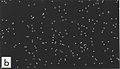  100 electrons
• 
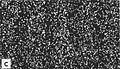  3000 electrons
• 
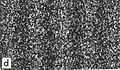  20000 electrons
• 
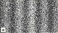  70000 electrons